FiduciaryVest Uses @RISK for Asset Allocation Modeling
Incorporating longer time horizons and probability functions associated with asset classes, analysts at FiduciaryVest were able to use @RISK to answer questions that cannot be addressed using static or optimized financial models.
“Using @RISK to get answers to these types of questions helps us give clients real-world insight into what to expect from their portfolio. More importantly, the models give our clients a strong indication of the impact that each component of asset allocation and diversification delivers in terms of their specific needs for future investment returns and risk management.”
Joe DiNunno, Insightful Ideas
Defining the Major Investment Challenge
Decision makers for all long-term investment pools face a critical challenge, regardless of their level of sophistication: Multi-year allocation among the various asset categories available to investors. This particular decision is known to be the primary factor that will determine long-term portfolio outcomes. Adequate investment management within the underlying asset class is actually a secondary issue. That being said, the inherent question is: How can asset allocation decisions be made with strong confidence that the outcomes will be appropriate to a particular client’s desired/expected financial needs? There are actually two challenges here: (a) Despite the simplicity of this statement of need, an adequate solution is complex; however, (b) the solution must be communicated to decision makers in user-friendly form that will be consistently understood.
The challenge can be met by assembling the following elements:
- A large volume of historical market and economic data that is well categorized and in significant detail.
- Significant investing knowledge and experience.
- Sophisticated software tools that are specifically designed for both historical pattern-identification and delivery of forecasted future outcomes, displayed in an easy-to-communicate graphic, probability format.
FiduciaryVest’s Approach
Joe DiNunno, of Insightful Ideas, and Gregg Buckalew, of FiduciaryVest, first started building asset allocation models that used the stochastic capabilities of @RISK in 1996. Today, DiNunno typically builds forecast models for several types of investment projects for clients: Custom Target Date portfolios, Defined Benefit Pension Plans (Including Asset/Liability (LDI)), Foundations/Endowments, and Hospital Balance Sheets.
FiduciaryVest’s asset allocation models are client-specific, and despite the high level of sophistication of these models, their clients do not need to have or acquire modeling expertise to contribute to them. Instead FiduciaryVest establishes each client’s preferences by discussing the following considerations with them:
- The time horizon for achieving the client’s defined investment objectives.
- A set of investment outcome goals within the client’s time horizon.
- A profile of the client’s risk tolerance, defined as exposure to “unacceptable outcomes” over the specified time horizon.
For those situations that require an asset/liability analysis, financial models may include projected cash flows such as: pension plan liabilities, annual foundation distributions, or hospital expenses. By adding liabilities to the modeling equation, the associates are able to determine, for example: (a) the probability of a participant reaching their retirement goals with a custom target date portfolio, (b) the probability of a foundation being able to meet its distribution requirements, (c) the probability of a defined benefit plan being able to meet its pension obligations, or (d) whether the combination of a hospital’s cash flow with its portfolio income will be enough to meet its financial obligations over the next five years. (This optional analysis may include working with a client’s record keeper, actuary, or hospital management consultant).
Why They Turned to @RISK
The traditional approach to asset allocation has been to use efficient frontier models that seek to find the optimal portfolio mix that has the lowest possible level of risk (standard deviation) for its level of return (mean). When all asset class returns are assumed to follow the normal distribution, an efficient frontier model will yield reward vs. risk results that are consistent with our simulation model over a one-year time frame. While this approach provides useful results, it still leaves many questions unanswered. This is where tools like @RISK and Monte Carlo simulation come into play.
To begin with, one feature of @RISK that DiNunno found very helpful in building financial models is its capacity to analyze historical data to determine a probability distribution for each asset class. Customarily, the normal distribution has been used to model asset classes. Using @RISK’s distribution fitting feature he found that, for example, both the income and total returns for bonds are better represented by the lognormal distribution than the normal distribution.
Another important motivation for choosing Monte Carlo simulation, in preference to the simpler optimization techniques of the efficient frontier model, is that it allows the user to realistically incorporate the effect of time horizons longer than one year. This is important because:
- if volatile assets like stocks are included in the model, then one-year modeling output has little chance of realism
- users of modeling output that includes stocks and other volatile assets should consider time horizons of at least 3-5 years
- @RISK’s probabilistic modeling output demonstrates to clients how multi-year time horizons increase the beneficial diversification effects of adding asset classes to the portfolio mix.
The Building Blocks Approach
The usefulness of any forecast (of anything) depends heavily on the quality of assumptions used to produce it. Beginning in 2000, DiNunno and Buckalew moved away from strictly historical returns-based assumptions for long range future behavior of the various asset classes, in favor of a “building blocks” approach. The foundation of all building blocks is the market-determined current risk-free interest rate, for the forward period that the client determines is its investing time horizon. Beginning with that risk-free rate, successive layers are added to reflect each investment category’s known historical risks (reflected in its range/randomness of returns) and the returns attributed to those risks. This method produces expected return premium characteristics for each asset class based on its historical pattern of returns relative to the risk-free rate, which makes the model’s assumption-set internally consistent and logical. For the remaining two assumptions needed in forecasting (the variability of each category’s expected return, i.e., its standard deviation, and its cross correlation with each of the other categories’ returns), DiNunno and Buckalew believe there is strong evidence to support an assumption that long-term history is the most reliable predictor for those two factors.
Individual asset-class return assumptions are thus driven by the projected risk-free rate of return over the investment time horizon. For example, as of January 2019 the model’s “foundation block.” for constructing the expected returns of all asset classes was a 1 to 2% risk-free rate. By comparison, the long-term historical risk-free rate has been 5 to 6%. The risk premium developed for each asset class is then added to this risk-free rate to build the expected return used in their models.
While the asset allocation model assumptions are updated on a regular basis to reflect current market conditions, the biggest change over many years has been the movement from models that included 5-6 potential asset classes within a client portfolio (i.e. bonds and stocks) to models that may now include more than 20 different asset classes for potential investment (i.e. real estate, hedge funds, and other alternative investments). It is a relatively straightforward technique to review a correlation matrix, in order to understand the diversification benefits of adding a single asset class to a portfolio of just stocks and bonds. On the other hand, getting a handle on the impact of escalating a portfolio of 5 or 6 asset class investments to a dozen or more requires a more robust analysis.
Lessons from the 2008 Finance Debacle
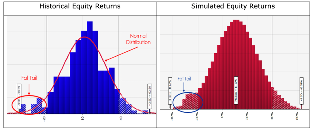
The financial crisis of 2008 convinced Joe and Gregg that it was time to look closer at the use of the normal distribution for modeling the probability of investment returns for equities. While the normal distribution assigns about 1 chance in 1000 for the stock market to experience a 3-standard-deviation decline, such as the market experienced in 2008, the reality is that a move of this magnitude occurs more frequently than that. Looking back at historical data, a move up or down of 3 standard deviations or more, over 6 months to a year, happens more like 2 out of every 100 time periods. The problem then is: How do you add ‘Fat Tails’ (outlier events that occur more frequently in reality than would be predicted by the normal distribution) to the model distribution in an effort to give the ‘theoretical’ stock market a more realistic chance of experiencing one of these ‘Black Swan’ events? The solution, as it turns out, was to use a combination of standard distributions that creates a simulated distribution that more closely resembles reality and provides more realistic ‘Fat Tails’.

Another revelation of the financial debacle in 2008 was the fact that correlations between most asset classes were, at least temporarily, much higher than expected. On the other hand, some asset classes that historically had a low correlation with equities had positive returns that year, a result that makes sense. With this in mind, DiNunno took a closer look at how correlations between asset classes have changed over time and more importantly under difficult circumstances. While some relationships were fairly consistent, others have been all over the map during the last 20 – 50 years. Since one of the major motivations for using financial modeling is to get a better handle on how a portfolio reacts when the financial system experiences a severe shock Joe decided to explore ways to incorporate stress scenario correlations into the FiduciaryVest asset allocation model.
Current Practice
The analysis of asset class correlations led to the recent addition of a 2nd correlation table in 2017 that is used by the asset allocation model during simulation runs when equity returns land in the lower left tail (extremely negative) of the return distribution. In this case the correlations between most asset classes are higher than in a normal financial market, but are lower for the few that often experience positive returns during significant drawdowns in equity investments. The result is a more realistic view of the risks that may be experienced by a specified investment portfolio.
DiNunno and Buckalew begin each client investment project with three important premises:
Premise 1: The forecasting of capital market outcomes is a reasonable exercise when the forecast is made for a future period of sufficient length to allow significant abatement of short-term randomness.
Premise 2: Fast-moving, exogenous market trauma, whether triggered by one-off acts of international terrorism, or sudden systemic failure in the capital market system, do not reduce the usefulness of multi-year mean/variance modeling output.
Premise 3: Although market events of 2008 were within the distribution range in FiduciaryVest’s previous modeling output, it is not within the model’s capability and purpose to attempt to forecast the timing of very low-probability occurrences (i.e., returns forecasted in the “tails” of model’s distribution output).
FiduciaryVest’s investment asset class assumption sets have a strong forecasting bias in favor of assumed central tendency, adjusted for the current cyclical stage at the time a portfolio model is created. The result is an internally consistent set of assumptions that run in a real-world modeling context to produce forecasted outcomes that are not only robust, but also practical for an average client decision-maker to understand and consider.
Incorporating longer time horizons and probability functions associated with asset classes, the colleagues were able to use @RISK to answer questions that cannot be addressed using static or optimized financial models:
- What is the probability of a negative return over a specific time period like 1 year, 3 years, 5 years, or 10 years?
- What is the probability of the client’s portfolio reaching (or not reaching) its targeted return over a given time period?
- What is the probability of meeting a client’s financial obligations without tapping into portfolio principal?
- What is the probability of a client’s participants reaching their retirement goals with a custom target date portfolio vs. a proprietary target date product?
DiNunno says: “Using @RISK to get answers to these types of questions helps us give clients real-world insight into what to expect from their portfolio. More importantly, the models give our clients a strong indication of the impact that each component of asset allocation and diversification delivers in terms of their specific needs for future investment returns and risk management.”
Read our Case Study on the Palisade Web Site.


